On Optimization -

A characteristic trait of humans, at least most of us, is the drive to solve problems. From the days of making spears with sharpened stones to the more recent efforts to develop brain-computer interfaces that enable monkeys to curse, humans have always sought to create tools to solve problems.

The intelligence problem is one that emerged approximately 70 years ago, non-coincidentally after the boom of the industrial revolution and the two world wars. We had mastered hardware. We had created sophisticated machines like industrial food manufacturing plants that essentially solved the hunger problem in many parts of the world. We had built machines capable of flying over a village, dropping death missiles with wanton grace and wiping out life within a 100 mile radius.

We had outdone ourselves.

All of these machines were however fully controlled by human intelligence from the bottom-up. It was clear that this constraint of being actively controlled by a human was a bottle-neck if we were ever going to squeeze more performance out of these machines. Therein began efforts to develop intelligence algorithms; algorithms capable of general problem solving and decision-making.

After 70 years of research on algorithms for intelligence, the emergent algorithms can be roughly grouped into 3 major classes:

Probabilistic Inference
Search
Optimization

Each of these classes of algorithms focuses on unique kinds of problems.

Probabilistic inference is often employed in problems where the probability of an event occurring is predicted given some form of evidence, prior knowledge or both. It is often invoked when there exists some form of uncertainty in the problem domain. Probabilistic inference is able to handle problems with either discrete variables, like the chances of getting a girlfriend given a person’s body odor, or continuous variables like the pose of a robot obtained from sensor fusion of the robot’s range readings and wheel odometry.

Search involves finding the sequence of actions to transition from some initial state to a target state. Search problems are often formulated as graphs of connected states, where each node in the graph represents a state and the edges between nodes represent the transition from one state to the other after an action is taken. The initial state and the goal state are often specified ahead of time. The goal of a search algorithm is often to find the shortest path between a start node and a goal node, often guided by some heuristic. Search is often used to solve discrete, combinatorial problems.

Optimization, or more specifically Mathematical programming is an approach for finding the optimal set of decision variables based on a specified objective function, that obey certain specified constraints.

Formally, Optimization problems are of the form

minimize $_x$ $f(x)$

subject to $g_i(x) \leq 0, i=1, ..., m$

where

$x \in R^n$ is the decision variable
$f:R^n \rightarrow R$ is the objective function
$g_i : R^n \rightarrow R$ are constraint functions

The feasible region of decision variables $C$ is a set whose elements satisfy all constraint functions. i.e. $C = {x : g_i(x) \leq 0, \forall i=1, ..., m}$ . The aim of an optimization function is to find the ‘best’ element $x^*$ in this region, where ‘best’ is decided by the objective function $f(x)$ ; essentially the value of $x$ that results in the least $f(x)$ across all $x$ ‘s in region $C$ .

Optimization algorithms can be used to solve problems with real or even integer decision variables that can be framed in terms of objective function and constraints. Solutions to optimization problems could either be global (the best possible) or local (the best within a local region) depending on the nature of the decision variables, the objective function or the constraint functions.

Optimization problems can be broadly classified into two groups:

Convex problems
Non-convex problems

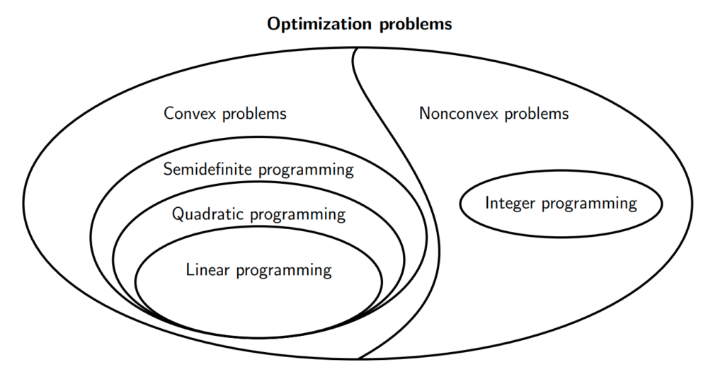
As noted in the figure above, there are different forms of convex and non-convex problems. The obvious question, is of course, what makes a problem convex?

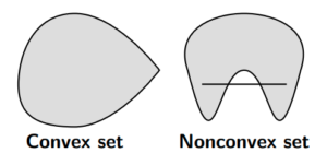
Formally, a set $C$ is convex if, for an $x,y \in C$ and $\theta \in [0, 1]$ ,

$\theta x + (1 - \theta)y \in C$

Intuitively, this means that if we take any two arbitrary elements in set $C$ and draw a line between them, all points on that line should also be elements in $C$ . This is pictorially demonstrated in the figure below:

Extending this definition to convex functions, a function $f : R^n \rightarrow R$ is convex if, for any $x, y \in R^n$ and $\theta \in [0, 1]$ ,

$f(\theta x + (1 - \theta)y) \leq \theta f(x) + (1 - \theta)f(y)$

This equation can intuitively be interpreted as,

To check for convexity of a function $f$ , take two arbitrary real numbers x,y , evaluate the function with these numbers as input to get points, $x, f(x)$ and $y, f(y)$ that lie on this function f. Draw a line to join these points. If this line lies strictly above the ‘valley’ of $f$ , then $f$ is convex. If this line lies strictly below $f$ , $f$ is concave. If the line intersects $f$ at multiple points, then $f$ is non-convex.

Convex optimization problems have convex objective functions, convex constraints and real-valued decision variables.

If either the objective function or constraint functions is non-convex, the problem becomes a non-convex optimization problem. Even if both objective and constraint functions are convex, a problem can be non-convex if its decision variables are not real-valued or continuous; i.e. integers. Such problems are called Integer Programming problems and are considered non-convex.

Some special cases of convex problems are:

Linear Programming: Objective function and constraint functions are affine (linear) functions. They have the form

minimize $c^T x + d$

subject to $Gx \leq h$

$Ax = b$

where $x \in R^n$ is the decision variable, $c \in R^n, d \in R, G \in R^{mxn}, h \in R^m, A \in R^{pxn}, b \in R^p$ .

Quadratic Programming: Objective function is a convex quadratic function whilst the constraints are all affine(linear). They have the form

minimize $\frac{1}{2}x^T Px + c^Tx + d$

subject to $Gx \leq h$

$Ax = b$

where all the symbols have the same definitions as in the linear programming form and $P$ is a symmetric positive semidefinite matrix. i.e. its eigenvalues $\geq 0$

Semidefinite Programming: They have the form

minimize $tr(CX)$

subject to $tr(A_i X) = b_i, i=1, ..., p$

$X \geq 0$

where the symmetrix matrix $X \in S^n$ is the optimization variable, the symmetric matrices $C, A_1, ..., A_p \in S^n$ are defined by the problem and the constraint $X \geq 0$ means that we are constraining $X$ to be positive semidefinite. $tr(.)$ is the trace function. (returns the sum of diagonal entries of the input matrix).

This concludes the overview of Optimization. In a future blog post (if my future self is still as bold to take on such a dragon), I will delve into methods for solving Convex Optimization problems and possibly look at code implementations for toy problems. And if my masochistic self is still unfazed by that dragon, I will subsequently delve into methods for solving Non-convex Optimization problems, particularly Mixed Integer Programming problems.

Oyasumi nasai.

Leave a Reply Cancel reply