On Convex Optimization -

Convex optimization problems form the bulk of optimization problems formulated in Robotics. Even though a bulk of the interesting optimization problems are indeed non-convex, it turns out that most of them can be approximated as convex problems given certain ‘relaxations’. This is convenient because there exist a plethora of capable and fast convex optimization solvers that can be easily applied to solve for global solutions to these convex relaxations. The results from these solvers often tend to be good enough to be used as solutions to the original non-convex problem.

Before providing a formal definition for convex optimization problems, we will first formally define convex sets and convex functions.

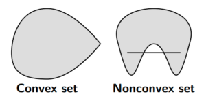
A set $C$ is convex if, for an $x, y \in C$ and $\theta \in [0,1]$ ,

$\theta x + (1 - \theta)y \in C$

Intuitively, this means that if we take any two arbitrary elements in set $C$ and draw a line between them, all points on that line should also be elements in $C$ . The figure below shows an example of one convex and one non-convex set.

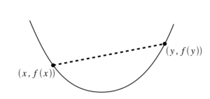
A function $f:R^n \rightarrow R$ is convex if its domain, $D(f)$ is a convex set and if, for all $x,y \in D(f)$ and $\theta \in R$ , $0 \leq \theta \leq 1$ ,

$f(\theta x + (1 - \theta)y) \leq \theta f(x) + (1 - \theta)f(y)$

Intuitively, this means that, if we pick any two points on the graph of a convex function and draw a straight line to connect them, the portion of the function between these two points will lie below this straight line, as pictured below.

A function is strictly convex if the definition for function convexity above holds with strict inequality for $x \neq y$ and $0 < \theta < 1$ . A function $f$ is concave if $-f$ is convex and strictly concave if $-f$ is strictly convex.

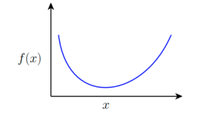
Some examples of univariate convex functions are Exponentials ( $f(x) = e^{ax}$ ), Negative logarithms ( $f(x) = -log x$ ), Affine functions ( $f(x) = b^Tx + c$ ), Quadratic functions ( $f(x) = \frac{1}{2}x^TAx + b^Tx + c$ ) where $A$ is symmetric matrix, etc.

Formally a convex optimization problem is an optimization problem of the form

minimize $f(x)$

subject to $x \in C$

where $f$ is a convex function, $C$ is a convex set and $x$ is the decision variable. A more specific formulation is

minimize $f(x)$

subject to $g_i(x) \leq 0, ~~ i = 1, \dots, m$

$h_i(x) = 0, ~~ i = 1, \dots, p$

To solve convex optimization problems, let’s first look at the unconstrained, one dimensional problem below

To find the minimum point $x^*$ , we know from basic calculus that this point is where the first derivative of the function, $f'(x) = 0$ . As expected, this condition is satisfied at the minimum point of $f$

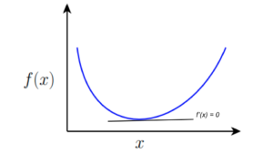
Generalizing for a multivariate function $f:R^n \rightarrow R$ , the gradient of $f$ must be zero

$\nabla _x f(x) = 0$

For simple enough convex objective functions where it is possible, simply compute $\nabla _x f(x)$ , set it to $0$ and solve for the optimal decision variable.

For more complex functions where it is not easy or possible to come up with an analytic expression for the first derivative $\nabla _x f(x)$ of the entire function, one could use either Gradient descent or Newton’s method to find the optimal decision variable.

Gradient descent proceeds iteratively by solving the gradient at a local region of the function and updating the value of the decision variable with a small multiple of the gradient. Thus, Repeat:

$x \leftarrow x - \alpha \nabla _x f(x)$

where $\alpha \in R > 0$ is a step size.

Newton’s method casts the problem as a root-finding problem to find a solution to the potentially nonlinear equation $\nabla _x f(x) = 0$ . Each iteration of Newton’s method subtracts from the current guess, the product of the inverse of the local hessian of $f$ with the local gradient of $f$ , evaluated at the current guess. i.e.

$x \leftarrow x - (\nabla ^2_x f(x))^{-1} \nabla _x f(x)$

Even though an iteration of Newton’s method is more expensive than an iteration of Gradient descent because of the inversion of the hessian, Newton’s method converges to the optimal decision variable in much fewer iterations than Gradient descent.

Now to the more interesting Constrained Convex Optimization problems…

There are a number of methods for solving Constrained Convex Optimization problems. I will describe a few of them below, as well as their trade-offs.

Active-Set method is used when the user has some way of knowing which constraints are active or inactive at each point in time. Active constraints are the equality constraints whilst inactive constraints are the inequality constraints. Knowing which constraints are active enables the user to solve the optimization problem by setting up a Lagrangian and solving the resulting equation using the Gauss Newton method. The active set method can be very fast if the user knows the active set before hand. Else, it can get nasty.

Barrier/Interior point method integrates the inequality constraints into the objective function by subtracting the logarithm of the constraint function from the objective function. This logarithm ensures that decision variable values that violate the constraint blow up the objective function value and as a result, encourages optimization to avoid such values.

minimize $f(x)$

subject to $c(x) \geq 0, i=1, \dots, m$

becomes

minimize $f(x) - \sum _{i=1} ^m \frac{1}{\rho} log (c_i (x))$

The Barrier method is the Gold standard for small-medium convex problems. It however requires a lot of hacks/tricks for non-convex problems.

Like the Barrier method, the Penalty method replaces inequality constraints with an objective term that penalizes violations

minimize $f(x)$

subject to $c(x) \geq 0, i=1, \dots, m$

becomes

minimize $f(x) + \frac{\rho}{2} [min(0, c(x))]^2$

Even though the Penalty method is easy to implement, it has issues with ill-conditioning and is difficult to achieve high accuracy.

The Augmented Lagrangian is an extension of the Penalty method that incorporates both equality and inequality constraints to the objective function, i.e.

minimize $f(x) - \lambda ^T c(x) + \frac{\rho}{2} [min (0, c(x))]^2$

Update $\lambda$ by offloading penalty term $\rho$ at each iteration.

The Augmented Lagrangian fixes the ill-conditioning of the Penalty method and converges fast to moderate precision. It also works well on non-convex problems.

These Constrained Optimization algorithms are often very tricky to implement. Most practical applications of these algorithms use either commercially available or open-source careful implementations of these algorithms. Being recent convert into the Julia cult, I’d highly recommend JuMP to anyone looking to do optimization. JuMP provides a great, intuitive and general interface to use all the various commercial and non-commercial optimization solvers out there. This link lists all the solvers that JuMP supports. This link will also lead you to tutorials on the JuMP website that provide really useful examples to get you familiar with the JuMP usage.

This ends my essay on Convex Optimization. My next post will potentially dwell on Mixed Integer Programming only because it has caught my fancy these past few weeks.

Oyasumi nasai.

Leave a Reply Cancel reply