Facts about Gaussian Processes
- Gaussian Process is a distribution over functions
- It is basically regression on steroids. It fits non-linear data and uses this to perform predictions on unseen data points
- It is non-parametric
- It is perfect for learning from a small amount of data
- It doesn’t scale well with large amounts of data though. This is because, it involves taking the inverse of matrices, which is an expensive procedure. Specifically

- The nice thing about Gaussian Processes is that they give explicit representation of the uncertainty of predictions through the covariance matrix. This way, if used in an active learning formulation, you’d know exactly how much confidence you can have in predictions in certain regions of the predicted function and which parts need more data to improve
Mathematical Formulation and Procedure for Noiseless Gaussian Process Regression
- Training data = X_train, f
- Test data = X_test
- We want to find f*, a distribution over y values for test data X_test
- We define a kernel function. Precisely, the Squared Exponential kernel.
- This kernel measures similarity between

- We first express f and f* as the joint probability P(f,f*)


- Where K is the similarity within X_train, as computed by the kernel function
 is the similarity between X_train and X_test
 is the similarity within X_test
- Using
 as defined above, we do 4 pages of linear algebra (the Sherman-Morrison-Woodbury formula. Details in Page 40 of this book) to get
- is defined by a Gaussian with mean
 and covariance matrix
  where
where
![\[\mu _* = K^T _* \cdot K^{-1} \cdot f ~~~and~~~ \Sigma _* = K^T _* \cdot K^{-1} \cdot K_{*} + K_{**}\]](https://alphonsusadubredu.com/wp-content/ql-cache/quicklatex.com-405858c36bfc961dfaedbef9892595e5_l3.png "Rendered by QuickLaTeX.com")
- When sampling from
 , use the Cholesky decomposition to find the square root of , L , where =
  . Sampling takes the form
![\[f_* = \mu _* + L \cdot \mathcal{N} (0,1)\]](https://alphonsusadubredu.com/wp-content/ql-cache/quicklatex.com-28e3b4f94693f91796d90b34e5d734c7_l3.png "Rendered by QuickLaTeX.com")
- f* is a distribution over “y-values” of X_test. And that’s the prediction we want from the learning done by training the GP.
Noisy Gaussian Process Regression
- Applying Gaussian noise

- Added noise only affects the covariance matrix. The new covariance matrix,
 becomes
![\[K_y = K + \sigma ^2 _y \cdot I_n\]](https://alphonsusadubredu.com/wp-content/ql-cache/quicklatex.com-8ad0c5e30e65d2b554e73a3cfff43ea4_l3.png "Rendered by QuickLaTeX.com")
- Hence the predicted distribution f_* is
![\[\mu _* = K^T _* \cdot K_y ^{-1} \cdot y ~~~and ~~\Sigma * = K_{**} - K^T _* \cdot K^{-1}\cdot K_{*}\]](https://alphonsusadubredu.com/wp-content/ql-cache/quicklatex.com-e10a4db3bcf5d83200b29cbbe29d7c49_l3.png "Rendered by QuickLaTeX.com")
Implementation from scratch in Python can be found in the link below, kind courtesy of Nando de Freitas’s Machine Learning course at UBC in 2013
Link to Python Implementation of Gaussian Processes
Simple implementations using the scikit-learn gaussian process library is below
import numpy as np
from matplotlib import pyplot as plt
from sklearn.gaussian_process import GaussianProcessRegressor
from sklearn.gaussian_process.kernels import RBF, ConstantKernel as C
from matplotlib import pyplot as plt
from sklearn.gaussian_process import GaussianProcessRegressor
from sklearn.gaussian_process.kernels import RBF, ConstantKernel as C
np.random.seed(1)
def f(x):
"""The function to predict."""
return x * np.sin(x)
"""The function to predict."""
return x * np.sin(x)
# ----------------------------------------------------------------------
# First the noiseless case
X = np.atleast_2d([1., 3., 5., 6., 7., 8.]).T
# First the noiseless case
X = np.atleast_2d([1., 3., 5., 6., 7., 8.]).T
# Observations
y = f(X).ravel()
y = f(X).ravel()
# Mesh the input space for evaluations of the real function, the prediction and
# its MSE
x = np.atleast_2d(np.linspace(0, 10, 1000)).T
# its MSE
x = np.atleast_2d(np.linspace(0, 10, 1000)).T
# Instantiate a Gaussian Process model
kernel = C(1.0, (1e-3, 1e3)) * RBF(10, (1e-2, 1e2))
kernel = C(1.0, (1e-3, 1e3)) * RBF(10, (1e-2, 1e2))
gp = GaussianProcessRegressor(kernel=kernel, n_restarts_optimizer=9)
# Fit to data using Maximum Likelihood Estimation of the parameters
gp.fit(X, y)
gp.fit(X, y)
# Make the prediction on the meshed x-axis (ask for MSE as well)
y_pred, sigma = gp.predict(x, return_std=True)
y_pred, sigma = gp.predict(x, return_std=True)
# Plot the function, the prediction and the 95% confidence interval based on
# the MSE
plt.figure()
plt.plot(x, f(x), 'r:', label=r'$f(x) = x\,\sin(x)$')
plt.plot(X, y, 'r.', markersize=10, label='Observations')
plt.plot(x, y_pred, 'b-', label='Prediction')
plt.fill(np.concatenate([x, x[::-1]]),
np.concatenate([y_pred - 1.9600 * sigma,
(y_pred + 1.9600 * sigma)[::-1]]),
alpha=.5, fc='b', ec='None', label='95% confidence interval')
plt.xlabel('$x$')
plt.ylabel('$f(x)$')
plt.ylim(-10, 20)
plt.legend(loc='upper left')
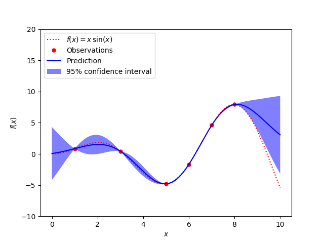
Plot of noiseless prediction and confidence interval
For noisy Gaussian Process Regression:
# now the noisy case
X = np.linspace(0.1, 9.9, 20)
X = np.atleast_2d(X).T
X = np.linspace(0.1, 9.9, 20)
X = np.atleast_2d(X).T
# Observations and noise
y = f(X).ravel()
dy = 0.5 + 1.0 * np.random.random(y.shape)
noise = np.random.normal(0, dy)
y += noise
y = f(X).ravel()
dy = 0.5 + 1.0 * np.random.random(y.shape)
noise = np.random.normal(0, dy)
y += noise
# Instantiate a Gaussian Process model
gp = GaussianProcessRegressor(kernel=kernel, alpha=dy ** 2,
n_restarts_optimizer=10)
gp = GaussianProcessRegressor(kernel=kernel, alpha=dy ** 2,
n_restarts_optimizer=10)
# Fit to data using Maximum Likelihood Estimation of the parameters
gp.fit(X, y)
gp.fit(X, y)
# Make the prediction on the meshed x-axis (ask for MSE as well)
y_pred, sigma = gp.predict(x, return_std=True)
y_pred, sigma = gp.predict(x, return_std=True)
# Plot the function, the prediction and the 95% confidence interval based on
# the MSE
plt.figure()
plt.plot(x, f(x), 'r:', label=r'$f(x) = x\,\sin(x)$')
plt.errorbar(X.ravel(), y, dy, fmt='r.', markersize=10, label='Observations')
plt.plot(x, y_pred, 'b-', label='Prediction')
plt.fill(np.concatenate([x, x[::-1]]),
np.concatenate([y_pred - 1.9600 * sigma,
(y_pred + 1.9600 * sigma)[::-1]]),
alpha=.5, fc='b', ec='None', label='95% confidence interval')
plt.xlabel('$x$')
plt.ylabel('$f(x)$')
plt.ylim(-10, 20)
plt.legend(loc='upper left')
plt.show()
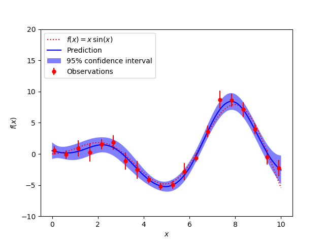
Plot of noisy prediction and confidence interval
My Thoughts
- Gaussian Processes are a neat way to learn from very little data
- I’m interested in using this, alongside other machine learning techniques to quickly learn skills needed for robots to perform long horizon reasoning through the learning of skills using very little data
- I was first introduced to Gaussian Processes from a paper about Active Model Learning and Diverse Action Sampling for Task and Motion Planning